Field Visualisation Options

The python/visualize_scenario_field.py helper renders solver field maps with a number of switches that mirror the "Visualization Upgrades" milestone from the roadmap.

Command-line summary

python3 python/visualize_scenario_field.py \
  --scenario inputs/two_wire_cancel.json \
  --field-map outputs/two_wire_field_map.csv \
  --draw-boundaries \
  --streamlines \
  --overlay-analytic interface \
  --vector-mode log \
  --vector-log-floor 1e-6 \
  --color-scale log \
  --log-floor 1e-6

Key options:

• --color-scale {linear,log} toggles between a linear palette and logarithmic magnitude scaling. Pair with --log-floor to bound the minimum |B| value.
• --draw-boundaries outlines material and magnet regions extracted from the scenario JSON so discontinuities are easy to spot.
• --outline-vtp PATH overlays solver-generated geometry outlines (domain, rotor assemblies, magnets, wires). When supplied, the helper automatically searches for the neighbouring _labels.csv metadata file so loop/group names can be joined in ParaView.
• --streamlines overlays streamlines traced from the field grid.
• --vector-mode {linear,log,off} controls the quiver arrows. The log mode compresses dynamic range using a log-normalised magnitude, while off disables the overlay entirely. --vector-log-floor mirrors --log-floor for the quiver transform.
• --overlay-analytic interface draws contour lines for the planar permeability interface analytic reference when available. Additional overlays can be added under the same flag in the future.
• --save PATH writes the rendered figure to disk; otherwise the viewer window opens interactively.

CI integration

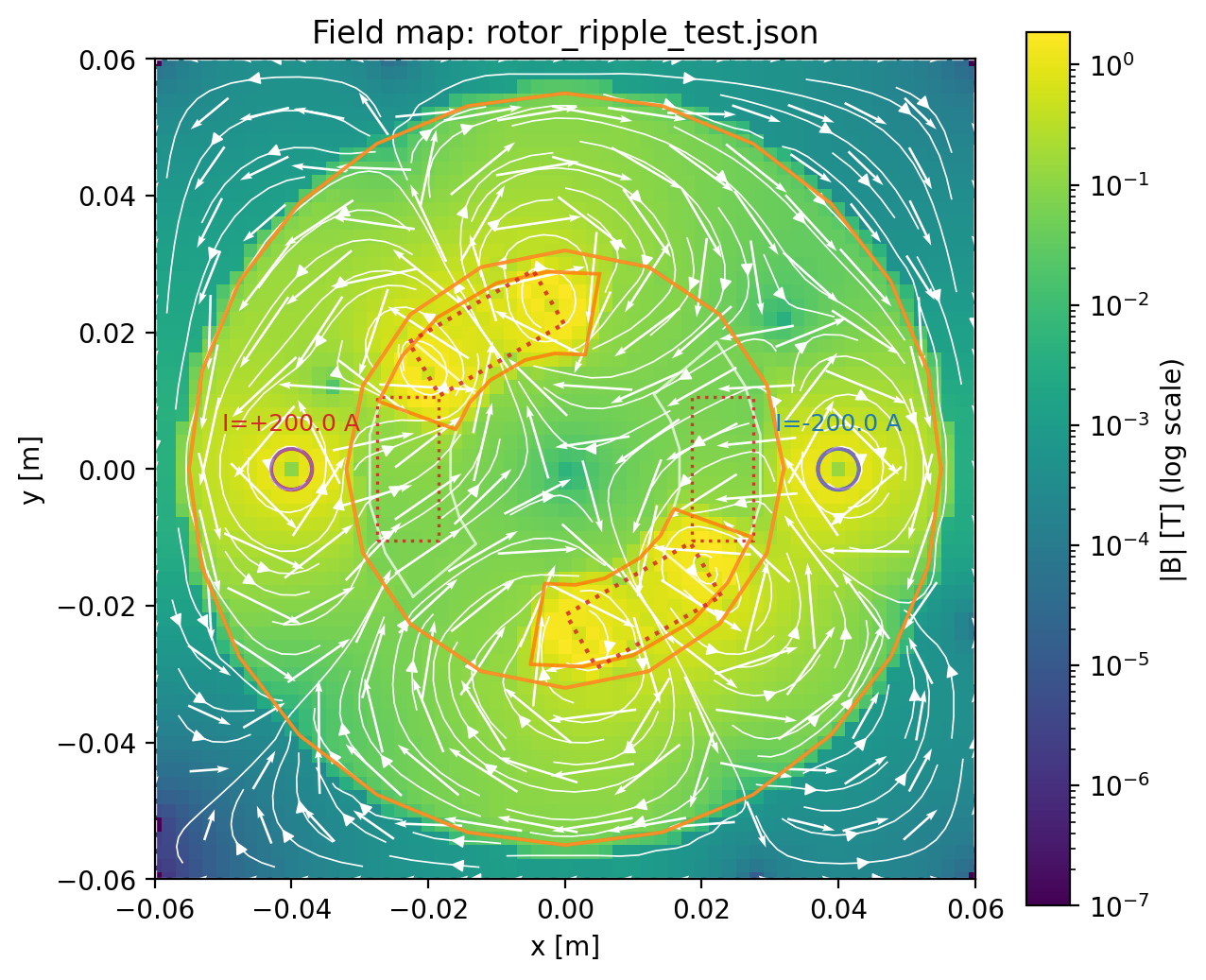
scripts/run_ci_checks.sh exercises these switches for the canonical demo scenarios so GitHub Actions artifacts include the enhanced renders. The iron ring and magnet strip plots use --color-scale log together with --vector-mode log to improve readability when the dynamic range spans several orders of magnitude, and the rotor ripple frames feed their per-frame _outlines.vtp files back into the renderer via --outline-vtp so the rotating rotor geometry is visible in the PNGs.

Rotor geometry animations

The new python/generate_rotor_animation.py helper renders rotor/stator motion using the geometry declared in a scenario JSON. It consumes the mechanical trace CSV (time, angle, speed) emitted by motor_sim and, when available, the circuit trace CSV (circuit_trace output) so stator slots can be coloured by their ampere-turns. Example invocation:

python3 python/generate_rotor_animation.py \
  --scenario inputs/dc_motor_spinup_ci.json \
  --rotor dc_rotor \
  --mechanical outputs/dc_motor_mechanical.csv \
  --circuit-trace outputs/dc_motor_currents.csv \
  --gif ci_artifacts/dc_motor_rotor.gif \
  --frame-png ci_artifacts/dc_motor_rotor.png

If a circuit trace is not supplied the script falls back to the timeline phase_currents data embedded in the scenario (useful for synchronous demos that prescribe the waveforms). When neither source is available the slots are rendered with neutral colours, still illustrating the rotor’s motion. The CLI supports frame limiting (--max-frames), alternate figure sizes, and PNG-only exports for quick smoke tests. CI runs this helper for the PM, induction, and DC motor demos so the uploaded artefacts include geometry-focused animations in addition to the full-field ParaView series.

ParaView overlays

When loading solver outputs directly in ParaView, open both the .vti field map and its *_outlines.vtp companion. The outline file carries cell data for the kind category and a loop_index, while the neighbouring *_outlines_labels.csv file provides the index-to-label mapping along with any rotor/stator group annotations. Join the CSV in the Spreadsheet view or an external tool to colour or filter geometry independently of the field. Select the B or H vector arrays for glyphs or streamlines—the data are already packaged as three-component vectors, so no calculator filters are required.

Open in GUI