Three-Phase Stator Scenario
This scenario bundles a six-slot, two-pole three-phase stator that drives a balanced rotating field. The Python generator produces both the tiny CI-sized case and a high-resolution configuration by tweaking a single profile flag.
Quickstart
python3 python/gen_three_phase_stator.py --profile ci --out inputs/three_phase_stator_ci.json
./build/motor_sim --scenario inputs/three_phase_stator_ci.json --solve --parallel-frames --vtk-series outputs/three_phase_ci.pvd --tol 5e-6 --max-iters 40000
python3 python/animate_three_phase.py --pvd outputs/three_phase_ci.pvd --scenario inputs/three_phase_stator_ci.json --save three_phase_demo.mp4 --frame-png three_phase_demo.png
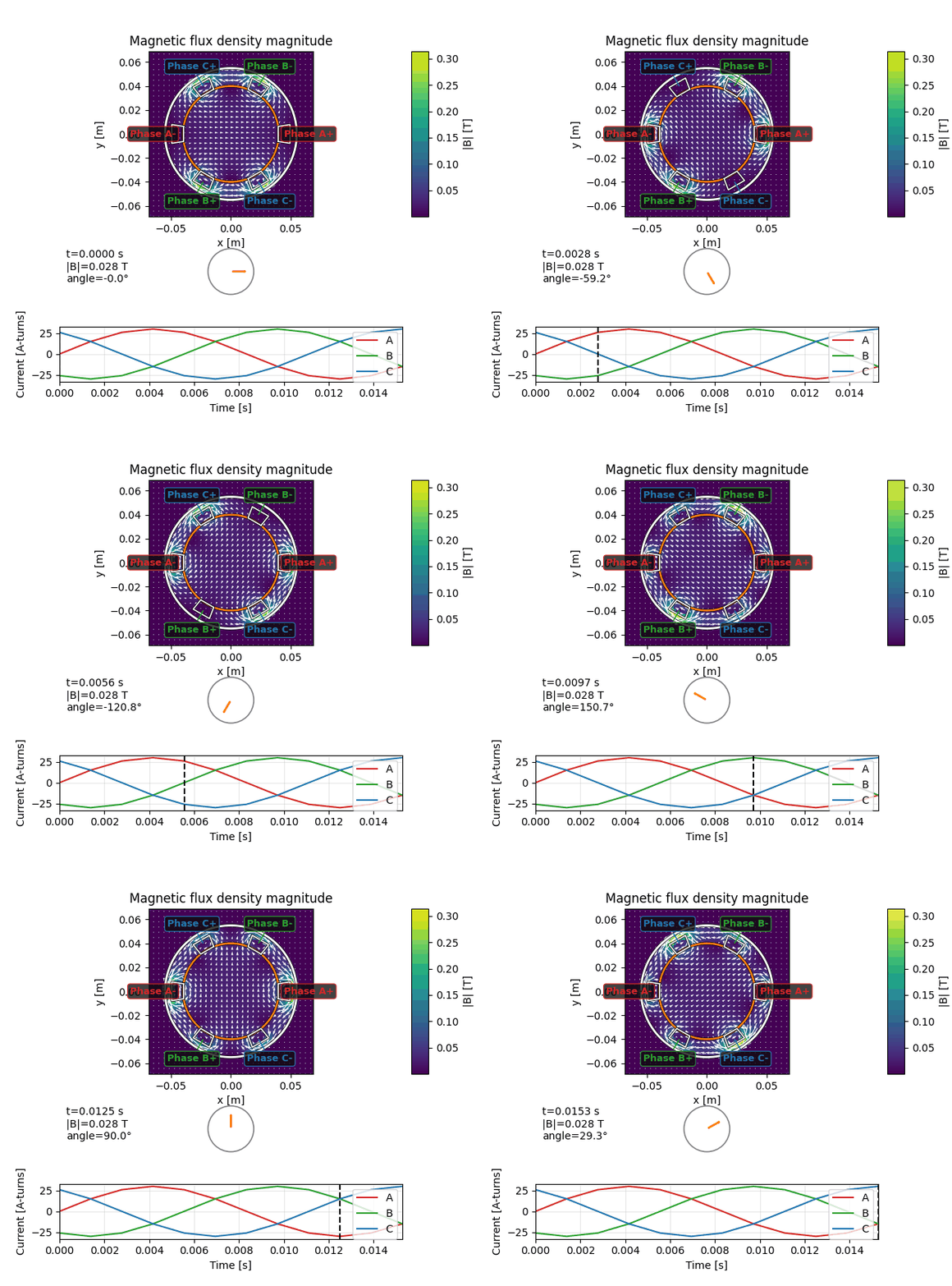
The generated scenario exports cell-centred VTK frames, a bore-average CSV, and polyline outlines that highlight the stator geometry.
Scaling up
The generator exposes two profiles:
ci: 65×65 grid, 12 frames (one electrical cycle)hires: 401×401 grid, 120 frames per cycle, three electrical cycles
Switch profiles via --profile hires to emit the high-resolution configuration.
All other pipeline steps remain unchanged—simply re-run motor_sim and the
animation command on the new JSON.
Outputs
outputs/three_phase_frame_###.vti: per-frame cell-centred B/H fields.outputs/three_phase_ci.pvd: ParaView time-series index (generated via--vtk-series).outputs/three_phase_outlines.vtp: geometry polylines for overlaying slot and stator boundaries.outputs/bore_angle.csv: bore-average B components, magnitudes, and angles.
ParaView tips
- Open the
.pvdseries to load the time-resolved field data. - Add
three_phase_outlines.vtpas a separate source and enable it in the pipeline to overlay slot and stator geometry. - Use the “Glyph” filter on
three_phase_outlines.vtpfor quick directional cues, or switch the VTI representation to “Surface LIC” for streamline-like visuals.
Animation
python/animate_three_phase.py renders a full-field animation that overlays the
cell-centred |B| map, quiver arrows, bore compass, labelled slot outlines, and
the driving phase currents. The CLI accepts:
--pvd: VTK time-series index produced bymotor_sim --vtk-series.--scenario: scenario JSON (required to extract timeline currents and bore polygon).--save: output path (MP4/GIF; binaries are uploaded as CI artefacts rather than committed).--fpsand--width: tune playback speed and output resolution.--html: emit an interactive HTML player (uses the same data as the MP4).--frame-png: write a static render of the first frame (handy for docs or quick inspection).--log-scale: switch the |B| colour map to logarithmic scaling to emphasise the field in low-magnitude regions.
The animation is designed for the CI demo case and remains lightweight enough for larger offline runs.
Notes
- The stator slots are modelled as polygonal
current_regionsources. Each slot carries 60 turns with a 0.55 copper fill fraction so the deposited ampere-turns match the intended winding pack without overdriving the bore field. The timeline provides per-frame phase currents via thephase_currentsblock. - With the default 30 A peak phase currents the CI profile’s bore probe reports roughly 0.03 T, so the rotating stator field remains visible when the PM motor rotor is introduced.
- The bore-average sanity check (
python/check_three_phase_field.py) unwraps the bore field angle, verifies monotonic rotation, enforces an R² > 0.95 fit against a straight line, and guards against magnitude collapse. The CI workflow runs it automatically. - Looking for a fully coupled permanent-magnet motor walkthrough? See
docs/three_phase_pm_motor.mdfor the rotor, circuit, and mechanical co-simulation demo. - Keep binary artefacts (MP4/VTI samples) out of git history. The CI workflow uploads a small bundle with the demo VTK frame, bore CSV, and animation.