Magnetostatic Solver Math Notes¶

This document summarizes the equations, discretizations, and validation strategy used by the minimal 2D magnetostatic solver implemented in this repository. It follows the scalar potential formulation with a single non-zero component \(A_z(x, y)\) and highlights practical implementation details for the structured grid solver. Reusable notation is collected under Reference → Equations.

1. Problem statement: 2D magnetostatics¶

We consider a 2D Cartesian cross-section where impressed currents are directed along the out-of-plane \(z\)-axis. The vector potential has only one non-zero component,

\[ \mathbf{A} = (0, 0, A_z(x, y)). \]

The magnetic flux density is recovered by taking the curl of \(\mathbf{A}\):

\[ \mathbf{B} = \nabla \times (0, 0, A_z) = \bigl(\partial_y A_z,\; -\partial_x A_z,\; 0\bigr). \]

Consequently,

\[ B_x = \partial_y A_z, \qquad B_y = -\partial_x A_z. \]

2. Governing PDE¶

Spatially varying materials are represented through the magnetic permeability \(\mu(x, y) = \mu_0 \mu_r(x, y)\). The scalar potential satisfies the Poisson-like equation

\[ \nabla \cdot \left( \frac{1}{\mu} \nabla A_z \right) = -J_z, \]

where \(J_z\) is the impressed current density in the \(z\) direction. In the special case of uniform permeability, \(\mu = \text{const}\), the equation reduces to

\[ \nabla^2 A_z = -\mu J_z. \]

3. Discretization on a uniform grid¶

The solver operates on a structured, uniform grid of size \((n_x, n_y)\) with spacings \(\Delta x, \Delta y\). All quantities are stored at cell centres:

\(A_z\): vector potential solution. In harmonic solves the code also stores an imaginary component \(A_z^{(i)}\).
\(J_z\): source term. A companion array stores the imaginary impressed current density when frequency-domain sources are used.
\(\nu = 1/\mu\): inverse permeability.
\(\sigma\): electrical conductivity (S/m), required for eddy-current calculations.

3.1 Variable-coefficient five-point stencil¶

Spatially varying materials require carefully averaging \(\nu\) across cell faces. Using harmonic averages preserves flux continuity across interfaces. For the east face shared by cells \((i, j)\) and \((i+1, j)\),

\[ \nu_E = \frac{2\,\nu_{i,j}\,\nu_{i+1,j}}{\nu_{i,j} + \nu_{i+1,j}}, \]

with analogous expressions for the west (W), north (N), and south (S) faces. These face coefficients yield the standard five-point stencil for diffusion with variable coefficients. The Gauss–Seidel point update used by the solver reads

\[ A_{i,j}^{(\text{new})} = \frac{ \tfrac{\nu_E}{\Delta x^2} A_{i+1,j} + \tfrac{\nu_W}{\Delta x^2} A_{i-1,j} + \tfrac{\nu_N}{\Delta y^2} A_{i,j+1} + \tfrac{\nu_S}{\Delta y^2} A_{i,j-1} + J_{i,j} }{ \tfrac{\nu_E + \nu_W}{\Delta x^2} + \tfrac{\nu_N + \nu_S}{\Delta y^2} }. \]

When \(\mu\) is uniform, \(\nu_E = \nu_W = \nu_N = \nu_S = 1/\mu\) and the update reduces to the familiar five-point Laplacian.

3.2 Discrete residual¶

The residual used for convergence checks is assembled directly from the fluxes through each face:

\[ R_{i,j} = \frac{\nu_E (A_{i+1,j} - A_{i,j}) - \nu_W (A_{i,j} - A_{i-1,j})}{\Delta x^2} + \frac{\nu_N (A_{i,j+1} - A_{i,j}) - \nu_S (A_{i,j} - A_{i,j-1})}{\Delta y^2} - J_{i,j}. \]

The continuous PDE is satisfied when \(R_{i,j} = 0\) everywhere.

4. Boundary conditions¶

The solver supports both Dirichlet and homogeneous Neumann boundary conditions on the outer rectangular boundary. Dirichlet fixes \(A_z = 0\), emulating a bounding conductor. Neumann enforces \(\partial_n A_z = 0\) so flux can exit without forcing a return through the box. In the Gauss–Seidel sweep the Neumann option mirrors the adjacent interior value into the boundary cell, making the forward difference for the normal derivative vanish.

5. Iterative solvers¶

The codebase exposes two matrix-free solvers that operate on the same discrete operator:

5.1 Gauss–Seidel with SOR¶

The legacy workhorse remains a Gauss–Seidel method with Successive Over-Relaxation (SOR). For every interior cell,

\[ A_{i,j}^{(\text{new})} = \frac{\tfrac{\nu_E}{\Delta x^2} A_{i+1,j} + \tfrac{\nu_W}{\Delta x^2} A_{i-1,j} + \tfrac{\nu_N}{\Delta y^2} A_{i,j+1} + \tfrac{\nu_S}{\Delta y^2} A_{i,j-1} + J_{i,j}}{\tfrac{\nu_E + \nu_W}{\Delta x^2} + \tfrac{\nu_N + \nu_S}{\Delta y^2}}. \]

Relaxation is applied as

\[ A_{i,j} \leftarrow (1 - \omega) A_{i,j} + \omega A_{i,j}^{(\text{new})}, \qquad 1 < \omega < 2. \]

SOR remains useful as a smoother and a robust fallback when diagnostics are required.

5.2 Preconditioned Conjugate Gradient (PCG)¶

For production runs the simulator now provides a preconditioned conjugate gradient solver tailored to the symmetric positive definite system. The PCG iteration is expressed in matrix-free form using the residual assembly routine shown earlier. Users can select a preconditioner at runtime via --pc {none|jacobi|ssor} (or the matching scenario schema). The Jacobi option applies the diagonal inverse of the operator, while the SSOR mode runs a matrix-free symmetric Gauss–Seidel sweep that respects the structured 5-point stencil. The update equations follow the standard PCG recurrence:

\[ \begin{aligned} r_k &= b - A x_k, & z_k &= M^{-1} r_k, & p_k &= z_k + \beta_{k-1} p_{k-1}, \\ \alpha_k &= \frac{r_k^T z_k}{p_k^T A p_k}, & x_{k+1} &= x_k + \alpha_k p_k, & r_{k+1} &= r_k - \alpha_k A p_k, \end{aligned} \]

with \(\beta_{k-1} = (r_k^T z_k) / (r_{k-1}^T z_{k-1})\). The implementation enforces Neumann symmetry by mirroring boundary values between iterations and monitors stagnation. If the relative residual fails to improve over a configurable window the solver emits guidance suggesting warm starts, prolongation, or falling back to SOR for inspection.

5.3 Transient magnetodynamics¶

Conductive regions introduce the magneto-quasistatic equation

\[ \sigma \frac{\partial A_z}{\partial t} + \nabla\cdot\left(\nu \nabla A_z\right) = -J_{\text{imp}}, \]

which, after linearising with a Crank–Nicolson step and assuming quasi-static magnetisation, yields the linear system

\[ \left(\frac{\sigma}{\Delta t}I + \mathcal{A}\right) A_z^{n+1} = \frac{\sigma}{\Delta t} A_z^n + J_{\text{imp}}^{n+1}, \]

where \(\mathcal{A}(\cdot) = -\nabla\cdot(\nu \nabla \cdot)\) is the same operator used in the magnetostatic solve. The implementation reuses the CG/PCG back-end by augmenting the matrix-free stencil with the \(\sigma/\Delta t\) diagonal term and supplying the adjusted right-hand side. Scenario JSON enables transient marching by adding a top-level "transient" block with dt and n_steps, and timeline frames advance sequentially so coupled circuit and mechanical subsystems remain synchronised with the EM state. The bundled diffusion regression (tests/diffusion_test.cpp) exercises this pathway and compares the recovered field against the analytic error-function solution for a step excitation into a half-space conductor.

6. Convergence criteria¶

Iterations continue until either the maximum iteration count is reached or the relative residual falls below the user-specified tolerance:

\[ \frac{\lVert R \rVert_2}{\lVert J \rVert_2 + \varepsilon} < \text{tol}, \]

with \(\varepsilon\) guarding against zero-current scenarios and the sums taken over all interior cells.

7. Recovering the magnetic flux density¶

Given \(A_z\), the magnetic flux density components are approximated via finite differences. In the interior we use central differences:

\[ B_x \approx \frac{A_{i,j+1} - A_{i,j-1}}{2\Delta y}, \qquad B_y \approx -\frac{A_{i+1,j} - A_{i-1,j}}{2\Delta x}. \]

One-sided differences are applied on the domain boundary where neighbours are unavailable.

8. Permanent magnets and magnetisation¶

Permanent magnets introduce a prescribed magnetisation \(\mathbf{M}(x, y)\) in addition to impressed current density. In the \(A_z\) formulation, magnetisation appears as an effective bound current density \(J_{m,z} = \partial_x M_y - \partial_y M_x\). The rasteriser stores uniform magnetisation vectors per cell and applies finite-difference curls to deposit this contribution into \(J_z\). The magnetisation field is also retained so that the magnetic field intensity can be reconstructed after the solve.

Given the flux density components, the solver supplies \(\mathbf{H}\) via

\[ \mathbf{H} = \nu \mathbf{B} - \frac{1}{\mu_r} \mathbf{M}, \qquad \nu = \frac{1}{\mu_0 \mu_r}. \]

In non-magnetised regions this reduces to the familiar \(\mathbf{H} = \nu \mathbf{B}\). Inside permanent magnets the subtraction cancels the remanent contribution, yielding nearly zero \(\mathbf{H}\) for an isolated uniformly magnetised body when \(\mu_r \approx 1\).

The magnet_strip_test regression models a rectangular magnet magnetised along \(+y\). The analytic reference treats the magnet as two opposing surface currents and integrates the Biot–Savart kernel along the strip edges. Numerical and analytic \(B_y\) agree to within 15%, and the recovered \(H_y\) inside the magnet is checked to remain near zero, validating both the bound current deposition and the post-processing of \(\mathbf{H}\).

With \(\mathbf{B}\) and \(\mathbf{H}\) reconstructed, the solver additionally evaluates the magnetostatic energy density

\[ w = \tfrac{1}{2} \mathbf{B} \cdot \mathbf{H} = \tfrac{1}{2} (B_x H_x + B_y H_y). \]

This scalar is emitted on request and supports energy-based force calculations or quick checks for material saturation.

9. Analytic reference: planar permeability interface¶

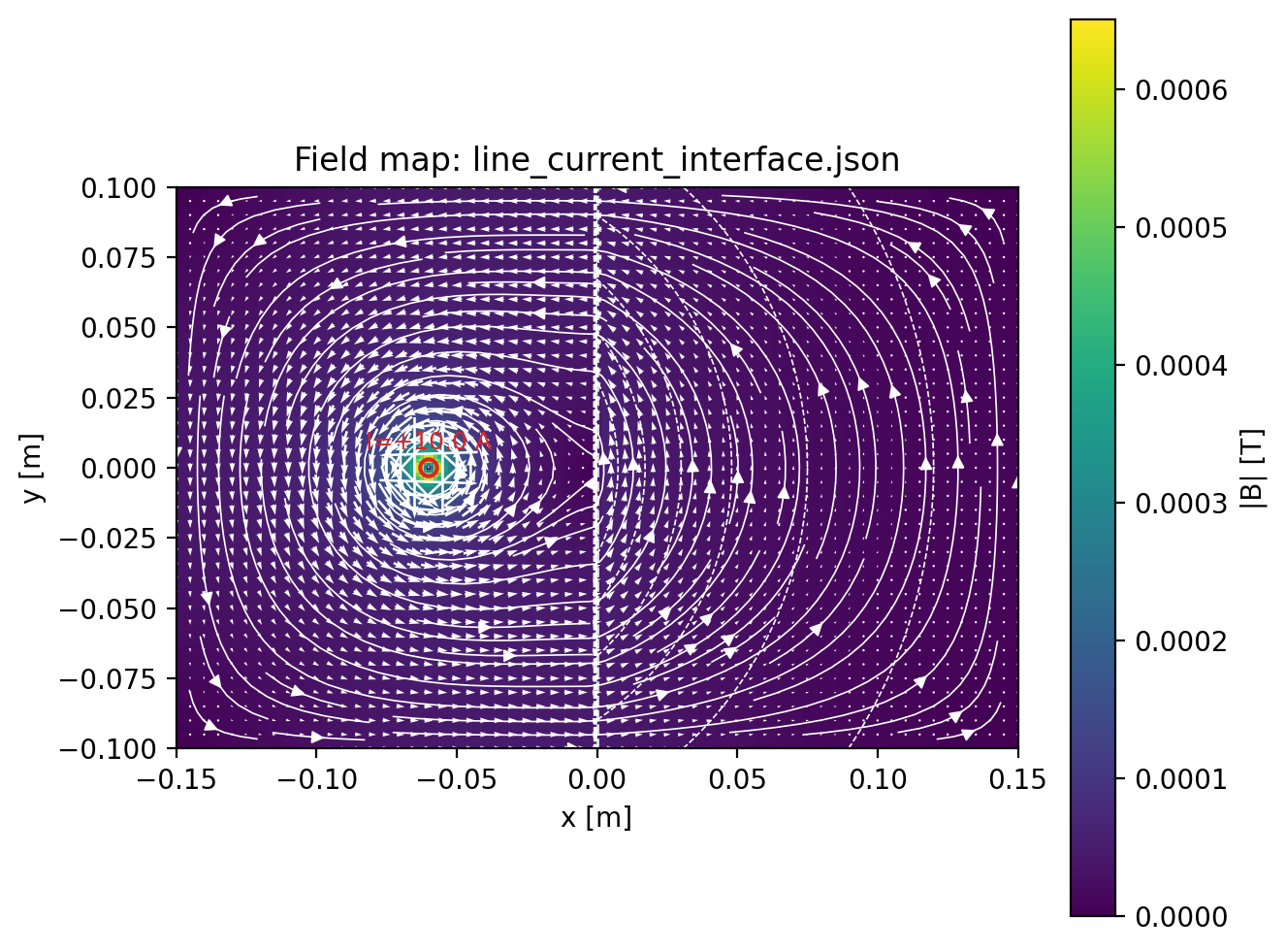
To validate heterogeneous permeability handling we leverage the method of images for a line current next to a planar interface. Two media with permeabilities \(\mu_1\) (left, \(x < 0\)) and \(\mu_2\) (right, \(x > 0\)) meet along the \(y\)-axis. A real infinite wire of current \(I\) sits at \(\mathbf{r}_0 = (-a, 0)\) inside region 1.

The magnetic field in region 1 is the superposition of the real wire and an image wire located at \(\mathbf{r}_0' = (+a, 0)\) with current magnitude scaled by

\[ I' = \rho I, \qquad \rho = \frac{\mu_2 - \mu_1}{\mu_1 + \mu_2}. \]

Region 2 sees the field of a "transmitted" wire that sits at the real location but carries current

\[ I_t = \tau I, \qquad \tau = \frac{2\mu_1}{\mu_1 + \mu_2}. \]

For a single infinite wire placed at \((x_s, y_s)\) inside a homogeneous medium with permeability \(\mu\), the Biot–Savart expression simplifies in 2D to

\[ \mathbf{B}(x, y) = \frac{\mu I}{2\pi R^2} \bigl(-(y - y_s),\; x - x_s\bigr), \qquad R^2 = (x - x_s)^2 + (y - y_s)^2. \]

Therefore the validation procedure assembles

Region 1 field: \(\mathbf{B}_1 = \mathbf{B}_{\mu_1}(I, \mathbf{r}_0) + \mathbf{B}_{\mu_1}(I', \mathbf{r}_0')\).
Region 2 field: \(\mathbf{B}_2 = \mathbf{B}_{\mu_2}(I_t, \mathbf{r}_0)\).

Sanity limits include \(\rho \to 0\) and \(\tau \to 1\) when \(\mu_1 = \mu_2\), \(\rho \to 1\), \(\tau \to 0\) when \(\mu_2 \to \infty\), and \(\rho \to -1\), \(\tau \to 2\) as \(\mu_2 \to 0\).

Simulated and analytic \(|\mathbf{B}|\) profiles along vertical probe lines in each half-space provide a sensitive regression on permeability contrast handling. The automated regression focuses on the air-side probe, where the relative error stays below 40% despite the coarse grid and Dirichlet boundary at the outer box.

Line current interface field

10. Validation with an infinite straight wire¶

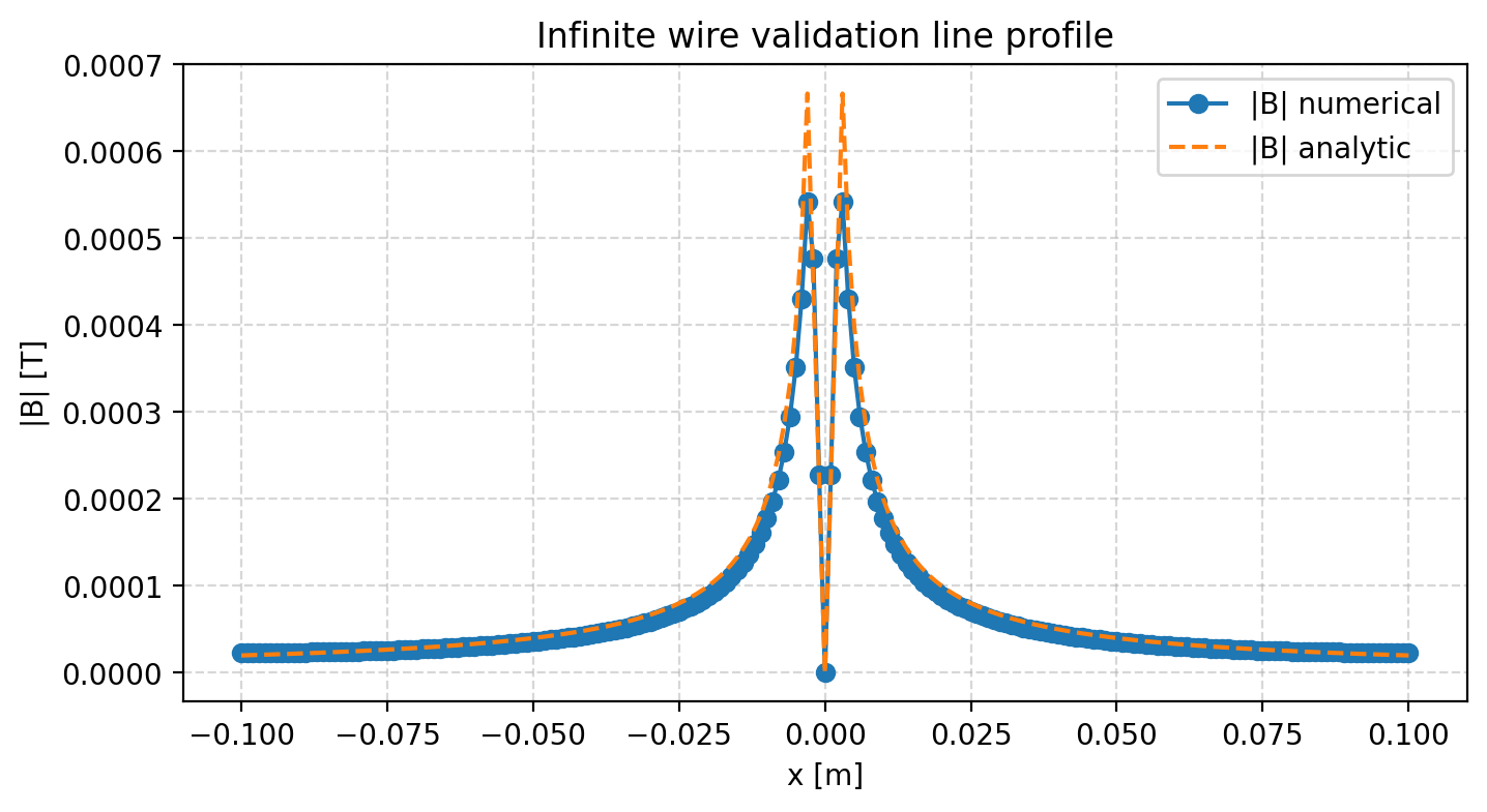
To validate the solver, we model an infinite straight wire carrying current \(I\). The analytic magnetic field magnitude is

\[ B(r) = \frac{\mu_0 I}{2 \pi r}. \]

Numerically, the wire is approximated by a small circular region (radius \(r_c\)) with uniform current density,

\[ J_z = \frac{I}{\pi r_c^2}. \]

Cells with centre radius \(r \le r_c\) receive this current density, while the rest are zero. Choosing \(r_c\) a few cells wide (e.g., three cell widths) reduces discretisation error from approximating the singular source. After solving for \(A_z\), we compute \(\mathbf{B}\) and sample points along a ring of radius \(r_{\text{sample}}\) to compare the simulated \(\lVert \mathbf{B} \rVert\) against the analytic expression. A relative error below 25% is deemed acceptable for the coarse grid and finite domain used in the automated test.

Analytic wire validation

This reference captures the mathematical foundations and numerical choices embedded in the minimal solver. Future extensions (e.g., alternative boundary conditions, conjugate gradient solvers, nonlinear materials) should extend these notes accordingly.

For runtime and scaling heuristics, consult docs/solver_performance.md, which summarises benchmark data from the bundled tooling.

11. Frequency-domain magneto-quasistatics¶

Conductive regions introduce eddy currents when the magnetic field varies in time. The simulator's first step toward induction modelling solves the steady-state magneto-quasistatic system for sinusoidal excitation. Assuming a phasor dependence \(e^{j\omega t}\) and a scalar potential \(A_z\) split into real and imaginary parts (\(A_z = A_r + j A_i\)), the governing equations become

\[ \begin{aligned} \nabla \cdot (\nu \nabla A_r) - \omega \sigma A_i &= J_r, \\ \nabla \cdot (\nu \nabla A_i) + \omega \sigma A_r &= J_i, \end{aligned} \]

where \(\sigma\) is the electrical conductivity and \(J = J_r + j J_i\) is the impressed current density. The discrete operator therefore couples the real and imaginary systems through the frequency-dependent \(\omega \sigma\) term.

The implementation keeps the matrix-free structure used by the magnetostatic solver. A helper applies the block operator

\[ \mathbf{H} = \begin{bmatrix} L & -\omega S \\ \omega S & L \end{bmatrix}, \]

where \(L\) is the familiar diffusion stencil and \(S\) holds per-cell conductivities. Because \(\mathbf{H}\) is not symmetric, the code forms the normal equations \(\mathbf{H}^T \mathbf{H} x = \mathbf{H}^T b\) and solves them with conjugate gradients. Dirichlet boundaries enforce the phasor gauge, and a Jacobi-like preconditioner can be added later without changing the interface.

Post-processing mirrors the magnetostatic pipeline: computeBHarmonic evaluates the complex curl of \(A_z\) to recover \(\mathbf{B}\), and computeHHarmonic applies \(\mathbf{H} = \nu \mathbf{B} - \mathbf{M}/\mu_r\) to obtain the magnetic field intensity phasor. The new materials[].sigma property, propagated through Grid2D::sigma, enables eddy terms while keeping legacy magnetostatic scenarios unchanged (\(\sigma = 0\)).

12. Scenario Spec v0.2¶

The solver ingests simulation descriptions authored as JSON documents. Version 0.2 extends the original schema with heterogeneous material regions while remaining backward compatible with 0.1 files. A valid document contains the following top-level members:

Field	Type	Notes
`version`	string	`"0.2"` preferred; `"0.1"` is still recognised for uniform-material scenarios.
`units`	string	`"SI"` only; currents in amperes, lengths in metres.
`domain`	object	`{Lx, Ly, nx, ny}` define the rectangular grid centred on the origin; `dx = Lx / (nx-1)` and likewise for `dy`.
`boundary`	object	Optional boundary condition override, e.g. `{ "type": "neumann" }`; defaults to Dirichlet when omitted.
`materials`	array	Each entry defines `{name, mu_r}` with unique names.
`regions`	array	Evaluated in authoring order. Entries may be `{"type": "uniform", "material": ...}` to set the background, `{"type": "halfspace", "normal": [nx, ny], "offset": c, "material": ...}` for planar masks, and `{"type": "polygon", "vertices": [[x1, y1], …], "material": ...}` to paint arbitrary simple polygons.
`sources`	array	Excites the field solve. Each entry is either a circular `{ "type": "wire", "x", "y", "radius", "I" }` or a polygonal `{ "type": "current_region", "vertices": [...], "I", "turns", "fill_fraction" }`.
`magnet_regions`	array	Optional list of magnetised shapes with uniform magnetisation vectors, e.g. polygon loops or axis-aligned rectangles.
`outputs`	array	Optional list of export requests. `field_map` records support `quantity` values `"B"`, `"H"`, `"BH"`, or `"energy_density"`; `line_probe` records accept `"Bmag"`, `"Bx"`, `"By"`, `"Hx"`, `"Hy"`, `"Hmag"`, or `"energy_density"`. All outputs are emitted as CSV.

loadScenarioFromJson validates the structure, normalises half-space normals, and stores the resulting material masks. rasterizeScenarioToGrid then deposits current density and inverse permeability onto a Grid2D. Later region entries override earlier ones so authors can compose layered masks (e.g. a uniform background followed by multiple half-spaces or polygons that carve out subdomains). Polygon masks use an even–odd rule on the provided vertex loop and honour region order, making it easy to emulate cut-outs (e.g. an outer iron annulus followed by an inner air bore).

The default CLI continues to wire these stages together:

JSON spec → ScenarioSpec → rasterise to Grid2D → solve A_z → compute B

Two helper layers keep authoring ergonomic:

python/scenario_api.py exposes dataclasses mirroring the schema and a Scenario.save_json() convenience. The API now includes a HalfspaceRegion primitive alongside the existing UniformRegion.
motor_sim --scenario path/to.json --solve [--list-outputs] [--outputs ids] loads the spec, solves the magnetostatic system, and emits any outputs declared in the JSON. Use --list-outputs to inspect available IDs and --outputs id1,id2 or --outputs none to control which requests are fulfilled at runtime. The legacy --write-midline flag remains available for ad-hoc dumps.

The sources list accepts both circular wires and polygonal current regions. wire entries remain a thin wrapper around the analytic Biot–Savart source: the rasteriser paints a disk of radius r with uniform current density J_z = I / (π r²) wherever the cell centre lies inside the loop. The tests/two_wire_cancel_test.cpp regression integrates the deposited density to confirm that it recovers the requested current to within 15% on the coarse CI grid.

current_region entries describe coil slots via arbitrary simple polygons. Each region stores an orientation (±1), optional phase label, the conductor current I, the number of turns threading the slot, and a copper packing factor fill_fraction. During rasterisation the simulator distributes the net ampere-turns evenly across the polygon,

J_z = (orientation × I × turns × fill_fraction) / area_polygon,

so that the integrated current density matches the requested ampere-turns even when the slot is only partially filled. The packing factor is clamped to [1e-4, 1] to avoid singular densities, and authors can drive the same slot from voltage-driven circuits (via coil links) or by prescribing timeline currents. tests/current_region_turns_test.cpp integrates the rasterised density and asserts the ampere-turn budget stays within 5% of the analytic value.

When a current region is driven by a coil_link, the circuit layer can override its effective orientation via a commutator object:

{
  "type": "coil_link",
  "inductor": "arm_L",
  "region": "armature_a",
  "turns": 110.0,
  "commutator": {
    "rotor": "dc_rotor",
    "default_orientation": 1.0,
    "segments": [
      {"start_deg": -90.0, "end_deg": 90.0, "orientation": 1.0},
      {"start_deg": 90.0, "end_deg": 270.0, "orientation": -1.0}
    ]
  }
}

At the start of each frame the circuit simulator normalises the associated rotor’s electrical angle, selects the segment whose [start_deg, end_deg) range contains it (wrapping across ±180° if needed), and multiplies the base region orientation by the selected orientation. The updated value is used for both current deposition and flux-linkage integration, letting commutated armatures flip polarity without editing the timeline geometry.

Magnetised regions live in magnet_regions; each entry supplies a shape (polygon with vertices or rect with x_range/y_range) plus a magnetisation vector magnetization given either as [Mx, My] or { "Mx": ..., "My": ... }. Overlapping entries add their vectors. Bound currents are generated from the resulting discrete curl, so partial coverage and composite magnets are supported.

Reserved future fields (e.g. a timeline array for time-varying studies) can be introduced without breaking the base schema because the parser ignores unknown members. Additional geometry primitives should extend the regions array with new type variants as needed.

10.1 Output requests¶

Output definitions live alongside the physical description so scenarios are self-documenting and reproducible. Two request flavours remain available:

Field maps ({"type":"field_map", "id":"domain_field", "quantity":"BH", "path":"outputs/domain_bh.csv"}) dump full-grid data. The CSV always starts with x,y and then includes whichever columns match the requested quantity: B (Bx,By,Bmag), H (Hx,Hy,Hmag), BH (both sets), or energy_density (both sets plus EnergyDensity). Paths default to outputs/<id>.csv when omitted.
Line probes ({"type":"line_probe", "axis":"x", "value":0.0, "quantity":"energy_density"}) sample a horizontal or vertical line aligned with the grid. Specify axis ("x" or "y"), the coordinate to lock, the field component (Bx, By, Bmag, Hx, Hy, Hmag, or energy_density), and an output path. The ingestor validates that the requested line lands on an existing grid column or row.
Mechanical traces ({"type":"mechanical_trace", "id":"pm_spinup", "rotors":["pm_rotor"]}) log rotor state samples after each solved frame. The CSV header is time_s,rotor,angle_deg,omega_rad_s,omega_rpm,torque_Nm, making it easy to validate spin-up behaviour or feed coupled ODE solvers during post-processing.

Python authors can build these records via scenario_api.FieldMapOutput/LineProbeOutput. Downstream tooling such as python/visualize_scenario_field.py consumes the emitted CSV to produce quick look plots for scenario debugging.